

Sample Size and Power Analysis for Metabolomics: Pilot Variance, Effect Size, Multiple Testing, and Biological Replicates
Submit Your InquiryA metabolomics study can be analytically successful yet statistically unable to answer its primary question. This usually happens when the sample count for a metabolomics project is selected from precedent, instrument capacity, or a fixed budget before the endpoint, experimental unit, expected effect, and analysis model are defined. The project may then generate thousands of technically acceptable features but insufficient evidence for the comparison that motivated the work.
The study claim, rather than a customary replicate count, sets the basis for sample-size planning. Ranking candidate pathways, estimating a treatment effect from a fixed panel, and modeling within-subject change are different statistical tasks. Each requires its own variance model, error criterion, and definition of a usable sample. There is no universal number of samples per group.
Study Objective, Primary Contrast, and Endpoint Definition
Power is the probability that a planned analysis will detect an effect of the specified magnitude when that effect is present. In metabolomics, the definition of "detect" changes with the claim. A study may be designed to detect one prespecified metabolite, identify a set of differential metabolites while controlling false discovery rate (FDR), estimate a multivariable classification performance, or demonstrate that a metabolic response exceeds a biologically relevant threshold. These are not interchangeable endpoints.
The planning conversation should resolve five items before any calculation is accepted:
- Primary contrast: Which comparison determines whether the study succeeds—treatment versus control, responder versus non-responder, pre- versus post-intervention, dose trend, or time-by-treatment interaction?
- Experimental unit: Is the independent unit a patient, animal, culture preparation, plant, plot, litter, organoid batch, or sampling occasion?
- Primary endpoint class: Is the outcome one named metabolite, a defined pathway score, a panel of quantified analytes, the global untargeted feature matrix, or a predictive model?
- Minimum relevant effect: What fold change, standardized difference, area-under-the-curve change, or prediction improvement would alter the scientific decision?
- Error criterion: Will success be judged by a nominal p-value, FDR-controlled discoveries, confidence-interval precision, or independent validation performance?
A calculation performed without these inputs may return a precise number, but the number has no defensible relationship to the study objective. For projects still refining the primary endpoint, the initial output should be a range of sample sizes across plausible scenarios rather than a single apparently definitive value.
| Study objective | Independent unit | Planning quantity | Appropriate output |
|---|---|---|---|
| Quantify change in one prespecified metabolite | Subject, animal, or independent culture | Expected mean difference and residual variance | Sample size for a defined confidence interval or hypothesis test |
| Screen an untargeted feature matrix | Independent biological sample | Effect-size distribution, feature variance, proportion of non-null features, and FDR target | Power curve or expected discovery rate across candidate sample sizes |
| Compare a targeted metabolite panel | Independent biological sample | Correlation among analytes, multiplicity strategy, and minimum relevant effects | Panel-level sensitivity under the planned correction rule |
| Estimate within-subject response | Subject with paired measurements | Variance of within-subject differences and within-subject correlation | Number of complete pairs plus allowance for incomplete follow-up |
| Develop a metabolic classifier | Subject, with all aliquots kept within the same partition | Event prevalence, model complexity, validation design, and optimism control | Development and locked-test sample requirements |
| Model repeated time points or dose response | Subject or experimental unit | Covariance structure, interaction effect, missing visits, and nonlinear trend assumptions | Simulation-based power for the prespecified mixed model |
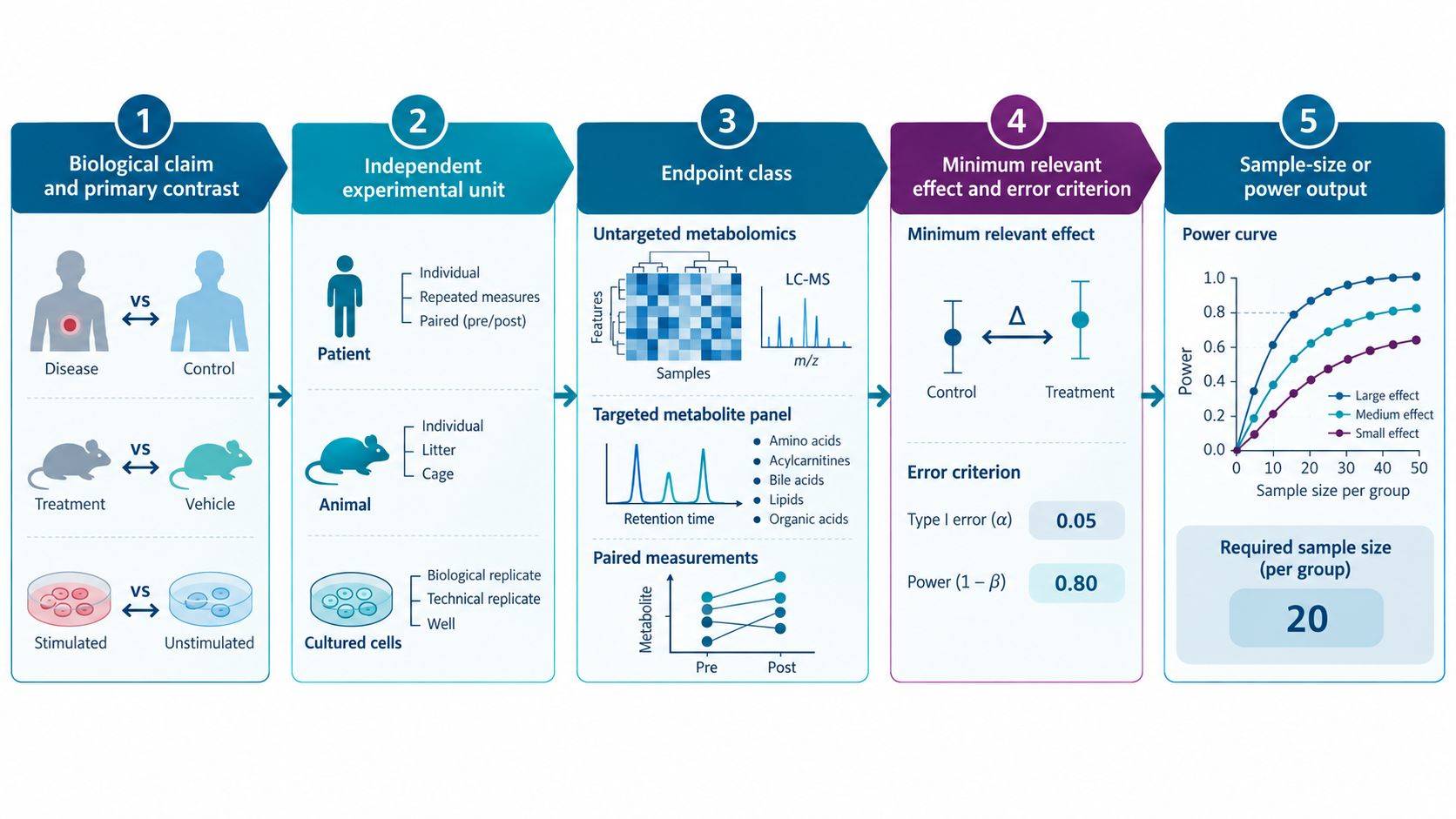 Figure 1. Metabolomics sample-size planning begins with the claim rather than a default replicate count. The primary contrast, independent experimental unit, endpoint class, effect threshold, and error criterion determine which variance estimate and power framework are appropriate.
Experimental Unit and Replication Structure
The most important number in a power analysis is the number of independent biological units, not the number of vials or injections. Repeated injections of one extract characterize analytical repeatability; they do not increase biological sample size. Multiple aliquots from the same patient, several wells seeded from the same culture preparation, or multiple tissue pieces from one animal are correlated observations unless the design and model explicitly treat their nesting.
Biological, Technical, and Analytical Replicates
- Biological replicates represent independently generated biological units and support inference to the target population.
- Technical replicates repeat sampling, extraction, or processing from the same biological unit and estimate variation introduced by those stages.
- Analytical replicates reinject the same prepared extract and primarily measure injection and instrument repeatability.
If biological variation is much larger than technical variation, allocating additional budget to biological samples usually produces more information than repeated injections. Technical replication remains useful during feasibility work, when extraction repeatability is unknown, when sample volume permits assessment of a critical processing step, or when the analytical signal is close to the limit of quantification. It should not be counted as independent evidence.
Pseudoreplication can create implausibly small p-values while leaving the effective sample size unchanged. A cell-culture study with three independent culture preparations and four wells from each preparation has three biological replicates, not twelve, unless wells were independently initiated in a manner that justifies that unit. Similarly, ten biopsies from one patient do not replace ten patients for a population-level claim. The sample manifest should identify subject, parent unit, collection event, aliquot, extraction batch, and injection so that the statistical model can preserve this hierarchy.
Paired-Design Efficiency and Missing-Pair Allowance
Paired designs can reduce residual variance because each subject acts as its own reference. The gain depends on the correlation between paired measurements and is lost when either member of a pair fails QC. Sample-size planning must therefore use the variance of the within-pair difference—not the variance of either time point alone—and include allowance for incomplete pairs. Randomization, extraction, and acquisition should also preserve the paired structure across batches rather than processing all baseline samples separately from all follow-up samples.
Pilot-Based Variance Estimation and Effect-Size Uncertainty
A pilot dataset is most valuable when it measures the variance components and operational losses expected in the main study. Small pilots are poor sources of a stable effect-size estimate: observed fold changes are highly variable and may be inflated by selection of the most promising features. Planning directly around the largest pilot effect can therefore understate the required sample size.
The pilot should use the intended matrix, collection procedure, storage conditions, extraction workflow, chromatography, ionization modes, and processing pipeline. At minimum, it should provide:
- the distribution of within-group variability after the intended normalization and transformation;
- the proportion of features retained after blank, missingness, dilution-linearity, and QC-variation filters;
- within-subject correlation for paired or longitudinal designs;
- variance attributable to extraction and analytical repeatability when technical replication is included;
- expected sample failure from insufficient volume, hemolysis, degradation, acquisition failure, or prespecified QC exclusions;
- class imbalance, event prevalence, or response frequency for clinical and predictive studies.
Variance should be evaluated for the endpoint that will actually be analyzed. Raw peak areas may have a strong mean–variance relationship; log transformation or another prespecified transformation can stabilize variance. For targeted absolute quantification, concentration uncertainty near the lower limit of quantification requires different treatment from variance in the central calibration range. For untargeted data, the pilot-derived feature matrix should pass the same filtering rules planned for the final analysis before its variance distribution is used.
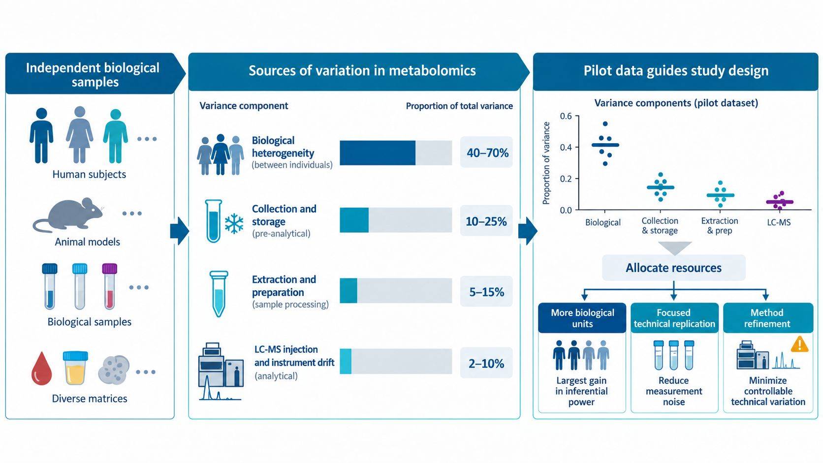 Figure 2. Variance observed in a metabolomics dataset combines biological heterogeneity with pre-analytical, extraction, and instrument components. A pilot study should quantify the components that can be controlled and establish whether budget is better allocated to additional biological units, technical replication, or method refinement.
Variance Assumptions Without Local Pilot Data
Planning can proceed without local pilot data, but uncertainty must be explicit. Suitable inputs, in descending order of relevance, include an earlier study using the same matrix and analytical workflow, a closely matched public dataset, a literature estimate for a prespecified metabolite, or a deliberately broad range of standardized effects and coefficients of variation. The result should be a sensitivity table: for example, the number required under low, moderate, and high variance, each evaluated at the minimum effect that would still be scientifically useful.
If the plausible range is too wide for a single-stage commitment, use an internal-pilot or staged design. An initial block can estimate nuisance variance and sample failure, followed by a blinded re-estimation of total sample size where the protocol and governance permit it. The rule for continuation, expansion, or redesign should be written before inspecting group-specific biological effects.
Power Models by Analytical Objective
Targeted Endpoints
For one prespecified metabolite, conventional power analysis may be appropriate when the planned statistical model and its assumptions are clear. A targeted metabolomics panel requires the same discipline at panel level: minimum relevant differences, residual variance, allocation ratio, significance threshold, and desired power must be tied to named analytes and a declared multiplicity rule. Paired, clustered, covariate-adjusted, and repeated-measure endpoints additionally require their correlation or covariance structure.
A targeted panel introduces multiplicity. Treating fifty metabolites as fifty independent primary endpoints at an unadjusted alpha of 0.05 does not preserve the intended false-positive rate. The protocol should distinguish primary metabolites from secondary or exploratory analytes and specify whether family-wise error, FDR, hierarchical testing, or a pathway-level summary is used. Power must be evaluated under that same rule.
Untargeted Discovery
Untargeted metabolomics datasets frequently contain thousands of correlated features, including isotopes, adducts, fragments, and multiple signals arising from the same metabolite. The raw feature count is not the number of independent biological hypotheses, but the scale of testing still requires explicit multiplicity control and generally more samples than a single-endpoint analysis.
Planning approaches may model the distribution of feature-level effect sizes and variances, the expected proportion of truly changing features, and the target FDR. Packages such as MetSizeR use pilot data and simulation to estimate sample requirements for high-dimensional metabolic phenotyping. These estimates remain conditional on the representativeness of the pilot, preprocessing choices, and assumed proportion of non-null features. A power curve across several sample sizes is more informative than reporting one number without its assumptions.
Prediction and Biomarker Models
Power to detect differential abundance is not the same as the sample requirement for a predictive model. Classification studies must reserve information for model selection, tuning, calibration, and honest performance evaluation. All aliquots and repeated measurements from the same subject must remain in one partition. Feature selection performed before cross-validation, or a random train–test split that leaks subject information, produces optimistic performance regardless of the nominal sample count.
The required sample size depends on outcome prevalence, the effective number of candidate predictors, expected discrimination, calibration requirements, and the validation strategy. When the cohort is modest, nested cross-validation can support model development, but it does not replace external validation. A project intended to claim clinical discrimination should budget separately for discovery and locked validation rather than using all available samples to maximize the initial area under the curve.
Multiplicity, Covariates, and Population Heterogeneity
Effect size and variance do not operate in isolation. Several design choices change effective power even when the nominal number of samples stays constant.
Multiple Testing and Discovery Thresholds
The threshold used in the final analysis must also be used in planning. Untargeted discovery commonly controls FDR rather than using thousands of unadjusted p-values. More stringent error control reduces false positives but raises the sample requirement for a given effect. Conversely, restricting the primary hypothesis set—through a predefined metabolite panel, pathway score, or staged discovery/confirmation workflow—can concentrate power on the question that matters.
Covariate Balance
Age, sex, body mass index, diet, fasting status, medication, microbiome-related exposures, genotype, circadian timing, and collection site can contribute variance or confounding. Covariate adjustment may improve precision when covariates are prognostic and measured reliably, but it cannot repair complete separation between biology and batch. Stratified randomization, blocking, or matching should be considered before acquisition. The power analysis should reflect unequal group allocation and major stratification factors rather than assuming perfectly balanced groups that will not exist.
Biological Heterogeneity
A tightly controlled cell model and a heterogeneous clinical cohort cannot share a replicate rule. Human cohorts often require larger sample sizes because inter-individual variation is substantial and the effects of interest are modest. Heterogeneity can sometimes be reduced through eligibility criteria or paired designs, but narrowing the population also narrows the inference. The planning document should state whether the goal is a controlled mechanistic comparison or a result intended to generalize across clinically relevant subgroups.
Batch and Center Effects
Adding samples across acquisition batches or clinical centers increases nominal sample size but can reduce usable information if batch is confounded with group. Each major biological group should be represented across batches, and bridge or reference materials should connect long acquisition series. If site or batch is included as a fixed or random effect, the number of levels and allocation within levels influence precision. One center containing only cases and another containing only controls leaves the biological contrast inseparable from center.
Budget Allocation Across Biological Replication and Analytical Scope
Budget decisions belong after variance and endpoint structure are defined. The lowest-cost option per injection may still be the least informative design if it reduces independent biological replication or omits measurements required for the primary endpoint.
| Constraint or observation | Preferred allocation | Reason |
|---|---|---|
| Biological variance dominates and analytical CV is acceptable | Increase independent biological samples | Additional injections of existing extracts do not improve population inference |
| Extraction repeatability is uncertain | Run a focused technical pilot before scaling | Method refinement may reduce variance across every subsequent sample |
| Sample volume is limited but the endpoint is prespecified | Prioritize a validated targeted assay | Concentrating analytical sensitivity on defined metabolites can be more efficient than broad profiling |
| Objective is hypothesis generation | Preserve biological diversity and untargeted coverage | Discovery value depends on representative biology and controlled false discoveries |
| Paired samples are available | Protect complete pairs and balance them across batches | Within-subject contrasts can reduce residual variance only when both measurements remain usable |
| Expected dropout or QC failure is material | Inflate recruitment or collection count before analysis | Replacing failed samples after unblinding can introduce bias and disrupt randomization |
| Several subgroups must support separate conclusions | Power each prespecified subgroup or interaction | A powered overall comparison does not guarantee an interpretable subgroup result |
A practical calculation distinguishes the analyzable sample requirement from the collection or recruitment target. If the main analysis needs a specified number of complete biological units, the collection target must additionally cover consent withdrawal, missing visits, insufficient volume, pre-analytical exclusions, extraction failures, and analytical QC failures. These losses should be estimated from relevant operations data rather than a generic percentage.
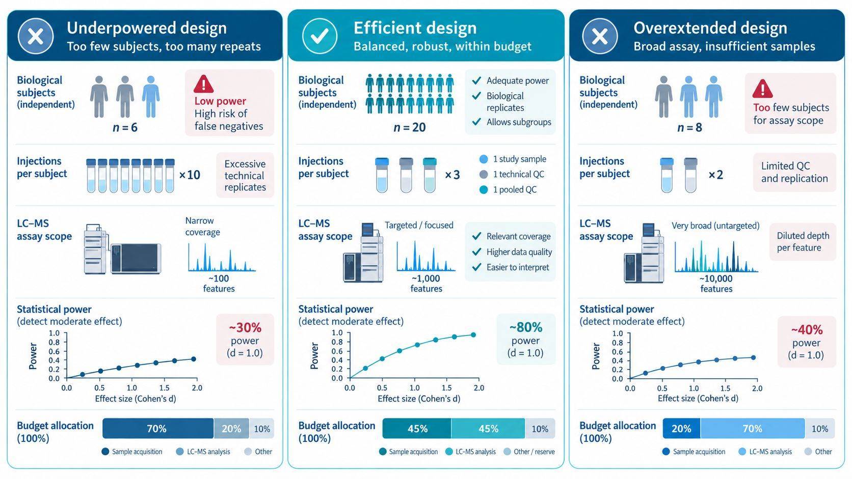 Figure 3. Fixed-budget planning should compare complete design scenarios rather than sample count alone. The preferred scenario protects independent biological replication, retains the measurements required for the primary claim, and includes realistic allowances for attrition and QC failure.
Sample-Size Assumptions and Sensitivity Scenarios
The planning record must allow a collaborator, statistician, or reviewer to reproduce the calculation without reverse-engineering it from the final results. It should contain:
- the primary biological question and primary contrast;
- the experimental unit and all nesting, pairing, blocking, and repeated-measure structures;
- the endpoint definition and planned data transformation;
- the minimum scientifically relevant effect or precision target;
- variance, correlation, and attrition inputs with their sources;
- the significance, FDR, or confidence-interval criterion;
- the intended statistical model and covariates;
- sample sizes across sensitivity scenarios, not only the selected scenario;
- the analyzable sample requirement and the larger collection target;
- the randomization, batch allocation, blinding, and QC structure;
- a contingency rule if pilot assumptions fail before full-scale acquisition.
For untargeted projects, the record must include preprocessing choices that materially affect power: blank filtering, missingness threshold, dilution-linearity criteria, QC-based feature filtering, normalization, transformation, and multiplicity correction. These choices need to match the planned metabolomics data analysis, because a calculation based on unfiltered pilot features cannot justify a final model built from a heavily filtered matrix. Targeted projects instead need the analyte panel, calibration model, quantification range, handling of values below the lower limit of quantification, and primary-versus-secondary endpoint hierarchy.
Frequently Asked Questions (FAQs)
Is three biological replicates per group sufficient for metabolomics?
Three replicates may reveal large effects in tightly controlled systems, but it is not a generally defensible default. The required number depends on the independent experimental unit, variance, minimum relevant effect, multiplicity, model, and desired power. A small pilot can characterize technical performance, but confirmatory inference usually requires a design-specific calculation and more biological replication.
Should budget be spent on more biological samples or repeat injections?
When instrument and extraction repeatability are already acceptable and biological variance dominates, additional independent biological samples generally contribute more inferential power. Repeat injections are valuable for diagnosing analytical instability or rescuing a questionable injection, but they do not increase the number of independent biological units.
Can a published metabolomics study provide the variance estimate?
Yes, if its population, matrix, collection procedure, platform, preprocessing, and endpoint closely match the planned study. Published summary statistics may omit batch and filtering details, so the resulting calculation should be treated as a scenario rather than a guaranteed estimate. Local pilot data are preferable when the matrix or workflow is novel.
How should sample loss be included?
First calculate the number of analyzable independent units required for the primary analysis. Then increase the collection or recruitment target using realistic rates for dropout, incomplete pairs, insufficient volume, pre-analytical exclusions, extraction failure, and analytical QC failure. Losses that are likely to differ by group require special attention because simple inflation does not remove selection bias.
Does an untargeted study always require more samples than a targeted study?
Not automatically, but untargeted studies usually face a larger hypothesis space, more missingness and annotation uncertainty, and FDR-controlled discovery objectives. A targeted study can be powered around a small number of prespecified metabolites, whereas untargeted planning must account for the distribution of effects and variances across many features. The appropriate comparison depends on the claim, not on the platform label alone.
Can sample size be re-estimated after a pilot phase?
It can be re-estimated using a prespecified internal-pilot or staged design when governance, blinding, and the statistical protocol permit it. Re-estimation should focus on nuisance parameters such as variance or attrition and should avoid selecting an inflated treatment effect after inspecting group differences. The adaptation rule should be documented before the interim data are reviewed.
References
- Bragazzi, N. L., et al. (2026). A priori sample size determination and power analysis in metabolic phenotyping and integrative metabolomics: an application framework based on a systematic review of literature. Metabolomics, 22(4), 104. doi:10.1007/s11306-026-02464-y
- Nyamundanda, G., Gormley, I. C., Fan, Y., Gallagher, W. M., & Brennan, L. (2013). MetSizeR: selecting the optimal sample size for metabolomic studies using an analysis based approach. BMC Bioinformatics, 14, 338. doi:10.1186/1471-2105-14-338
- Blaise, B. J., Shintu, L., Elena, B., Emsley, L., Dumas, M. E., & Toulhoat, P. (2009). Statistical recoupling prior to significance testing in nuclear magnetic resonance based metabonomics. Analytical Chemistry, 81(15), 6242–6251. doi:10.1021/ac9007754
- Billoir, E., Navratil, V., & Blaise, B. J. (2015). Sample size calculation in metabolic phenotyping studies. Briefings in Bioinformatics, 16(5), 813–819. doi:10.1093/bib/bbu052
- Ivanisevic, J., & Want, E. J. (2019). From samples to insights into metabolism: uncovering biologically relevant information in LC-HRMS metabolomics data. Metabolites, 9(12), 308. doi:10.3390/metabo9120308
- Alseekh, S., et al. (2021). Mass spectrometry-based metabolomics: a guide for annotation, quantification and best reporting practices. Nature Methods, 18, 747–756. doi:10.1038/s41592-021-01197-1
- Saccenti, E., Hoefsloot, H. C. J., Smilde, A. K., Westerhuis, J. A., & Hendriks, M. M. W. B. (2014). Reflections on univariate and multivariate analysis of metabolomics data. Metabolomics, 10, 361–374. doi:10.1007/s11306-013-0598-6
- van Iterson, M., van de Wiel, M. A., Boer, J. M., & de Menezes, R. X. (2013). General power and sample size calculations for high-dimensional genomic data. Statistics in Applications in Genetics and Molecular Biology, 12(4), 449–467. doi:10.1515/sagmb-2012-0019

 Contact Us


